Introduction

Deep Learning research is gruelling.

You need to get the data, preprocess it, tune a bazillion different hyperparameters just well enough so your loss decreases just fast enough, and look at the loss bar for hours on end as your entire life flashes before your eyes.

Deploying this shiny, new model into production can seem a relatively straightforward task.

“Bah!”, you may say. “I’ll just make a flask server, pass the inputs to the model, and be done with it!”

But that, my friend, would not just be bad practice, it would come with a whole host of disadvantages:

1. Scalability: It would take a whole lot of work for it to work well with large models.

2. Speed: Python based backend servers are slow.

3. Hassle: If you updated the model after training it to be X% better, you would need to restart the server again - and downtimes can be horrendous in production.

4. Portability: Additional work, like writing gRPC and REST APIs, would be required to make it run on different devices.

And many many more. Making a robust, production-ready backend server suited to deploying Deep Learning models on your own will take a ton of time.

Hmm… so… what if.. there was… already… something… somewhere…

So… Tensorflow Serving, huh?

Tensorflow Serving, a part of the TensorFlow Extended (TFX) ecosystem, is a framework for deploying TensorFlow models as a service.

At the highest level, Tensorflow serving allows you to provide the necessary inputs to your model server, and return the model output.

Tensorflow serving provides both a REST API and a gRPC interface for you to interact with the deployed model. It also provides a whole host of features that make deployment smooth sailing:

1. Tensorflow serving is blazing fast for Tensorflow models.

2. It provides zero downtime model updates.

3. It works swimmingly with large models too.

4. You can deploy multiple versions of the same model.

5. You can deploy multiple models on the same server, with zero performance loss.

and many other features! For a more detailed look at what Tensorflow Serving provides, check out the detailed guide to Tensorflow Serving.

But there are some caveats.

1. Tensorflow Serving requires the model to be in Tensorflow’s SavedModel format, so you’ll have to convert your model to a Tensorflow model before you can deploy it. I suggest looking at ysh329/deep-learning-model-convertor for a simple tool to convert between various model types.

2. Tensorflow Serving currently only works on ubuntu. This is why the recommended way to run tensorflow serving is on a docker container. However, you are out of luck if you are on an Apple M1 Machine, because tensorflow does not work with Docker on M1.

Enough with the boring stuff. How does it actually work in real life? Let’s dive into an example where we will use Tensorflow Serving to deploy a single, and then multiple Tensorflow models behind a single server.

Getting hands-on

The Models

We start by downloading and extracting two pre-trained tensorflow models available on tfhub.

1. Magenta’s Fast Style Transfer for Arbitrary Styles, which takes an input image and a style image, returning the input image painted in the style of the style image (i.e. a stylized image).

2. Enhanced Super Resolution GAN, which generates a 4x higher resolution image from a lower resolution image.

The setup

We are going to make this as platform independent as possible, so we will be using the tensorflow/serving docker image, instead of installing tensorflow serving directly on our system.

Docker

Docker allows us to run an application/service in an isolated environment (called a docker container). The environment (called a docker image) contains everything required for the application/service to run, down to the operating system.

This is precisely what allows us to run tensorflow serving in any OS, since the tensorflow/serving docker image is built on top of an ubuntu image, which means that the tensorflow serving container will actually run on ubuntu no matter what OS you are on.

The container that we build is isolated from the host system (i.e. the system we are running docker on), so docker provides us ways to communicate in real time with the host system: port forwarding, volume mounts, and other features.

So if an API server is running on port 3000 inside the docker container, we will have to forward it to a port on our host system in order to make the API requests from the host system.

The actual set up

First we make sure we have docker installed, and install it if we don’t.

We’ll need to pull the latest tensorflow serving image from docker hub.

1

docker pull tensorflow/serving

Now if we do:

1

docker ps

to see what images we have installed, we should see the tensorflow/serving image.

Without docker (not recommended)

If for some reason you do not want to install docker, and are on an ubuntu system, you can install tensorflow serving with the following command:

1

apt-get update && apt-get install tensorflow-model-server

Model directory setup

We’ll put the models we downloaded earlier inside a directory called models. Tensorflow serving uses a fixed directory organization structure, where each model’s files should be stored in a directory {model_name}/{version}.

Our directory organization is as follows:

1
2
3
4
5
6
7
8
9
10
11
12
13
14
15
16

models
├── esrgan_super_resolution
│   └── 1
│       ├── saved_model.pb
│       └── variables
│           ├── variables.data-00000-of-00001
│           └── variables.index
│           
└── magenta_image_stylization
    └── 1
        ├── assets
        ├── saved_model.pb
        └── variables
            ├── variables.data-00000-of-00002
            ├── variables.data-00001-of-00002
            └── variables.index

i.e. the assets/, variables/ and *.pb files of the model should all be in the {model_name}/{version} directory. In this particular example, the version happens to be 1.

And we’re all set up! Let’s run the server, and serve our models!

Serving our model

Let’s start by serving only the stylization model first. We’ll make sure we are in the directory that contains our models folder, and run the command:

1
2
3
4

docker run -t -p 8501:8501 \
    -v "$(pwd)/models/magenta_image_stylization:/models/stylization/" \
    -e MODEL_NAME=stylization \
    tensorflow/serving

For those of you not versed in docker, this is what the flags in the above command do:

1. -p: tells docker to forward the port 8501 to the container port 8501, so that we can access the API from the host system. Tensorflow serving exposes the REST API on port 8501 inside the container, and a gRPC API on port 8500. We are currently only forwarding the REST API port 8501 here, so the gRPC API will not work on the host machine.
2. -v: tells docker to mount the directory models/magenta_image_stylization inside the container to the directory /models/stylization. Since -v takes only absolute paths, we are prepending $(pwd), the absolute path to the current directory we are in.
3. -e: tells docker to set the environment variable MODEL_NAME to stylization, so we can identify the model we are serving.

And viola! Our model server is up and running!

API

Now that our server is up, let’s have a look at what we can do with it.

Tensorflow Serving provides both gRPC and REST client APIs. Here we will look at the more popular REST API, since that is what most applications will be using.

Tensorflow serving provides APIs for:

Model Status

A simple status check, that returns the status of the model, behind the endpoint:

1

http://host:port/v1/models/{MODEL_NAME}

For our example, the endpoint will be:

1

http://localhost:8501/v1/models/stylization

Let’s perform a GET request, and look at what the response contains:

1
2
3
4
5
6
7
8
9
10
11
12

{
    "model_version_status": [
        {
            "version": "1",
            "state": "AVAILABLE",
            "status": {
                "error_code": "OK",
                "error_message": ""
                }
        }
    ]
}

Self explanatory, isn’t it? Our model, version 1, is available for serving, and is indeed OK!

Model Metadata

The metadata for the model. This is a pretty important if we are deploying models made by someone else, whose parameters we don’t exactly know (which is exactly what we are doing right now).

We simply add /metadata to the model status endpoint to get the endpoint for the model metadata, i.e.

1

http://localhost:8501/v1/models/stylization/metadata

Upon performing a GET here, our model metadata in JSON.

Of particular concern to us are the inputs of the model. We haven’t even looked at how the stylization model works yet!

The good thing, however, is we don’t have to know how it works. We do need to know the inputs for the model, however. And this gives us just that.

The response["metadata"]["signature_def"]["signature_def"]["serving_default"]["inputs"] will show us:

1
2
3
4
5
6
7
8
9
10
11
12
13
14
15
16
17
18
19
20
21
22
23
24

{
    "placeholder": {
        "dtype": "DT_FLOAT",
        "tensor_shape": {
            "dim": [{"size": "-1","name": ""},
                    {"size": "-1","name": ""},
                    {"size": "-1","name": ""},
                    {"size": "3","name": ""}],
            "unknown_rank": false
        },
        "name": "serving_default_placeholder:0"
    },
    "placeholder_1": {
        "dtype": "DT_FLOAT",
        "tensor_shape": {
            "dim": [{"size": "-1","name": ""},
                    {"size": "-1","name": ""},
                    {"size": "-1","name": ""},
                    {"size": "3","name": ""}],
            "unknown_rank": false
        },
        "name": "serving_default_placeholder_1:0"
    }
}      

We have quite a lot of information here!

We know that the model has two inputs: placeholder and placeholder_1.

And we know that the model inputs are of type float and have 4 dimensions. This will come in handy when we send requests to the API.

response["metadata"]["signature_def"]["signature_def"]["serving_default"]["outputs"] will give a similar response that lets us see the data type and shape.

We could have figured all this out by loading the model onto a python script and running model.summary() but this is so much easier!

The Regress/Classify and the Predict APIs

The Regress/Classify APIs are used as an interface for performing regression and classification tasks, while the predict APIs, are used for performing inference.

Their endpoints are similar to the model status endpoint, but with the addition of the :regress, :classify or :predict suffix. These are POST endpoints, so we’ll have to make a POST requests to them with the model input data in the body.

For regression or classification:

1

http://localhost:8501/v1/models/stylization:(regress|classify)

which obviously won’t work for our stylization model, since it is a prediction task, not a regression/classification task.

And

1

http://localhost:8501/v1/models/stylization:predict

for prediction, which is the endpoint we need for performing stylization

The predict request/response format

The POST request body for the regress/classify/predict APIs should be a JSON of the following form: (shamelessly yanked from the docs)

1
2
3
4
5

{
  "signature_name": "<string> (optional parameter)",
  "instances": "<value>|<(nested)list>|<list-of-objects> (use this if the input is in row format, else use 'inputs' and omit this parameter)",
  "inputs": "<value>|<(nested)list>|<object> (use this if the input is columnar, else use 'instances' and omit this parameter)"
}

And we will recieve a response of the form:

1
2
3

{
  "predictions": "<value>|<(nested)list>|<list-of-objects>"
}

with our predictions. If this seems a little confusing now, don’t worry, it will be cleared up by the example below.

So now we have all the building blocks we need to make a stylization application that makes use of our server. We can send input objects to the model and get output objects, corresponding to the prediction.

Let’s now see how a python client for this server would be!

Example Client Notebook

The source code for this article is available on github, btw

Importing modules to load, transform the image, and send prediction requests to the API

1
2
3
4

import cv2
import requests
import numpy as np
import matplotlib.pyplot as plt

Global Variables

The STYLE_MODEL_IMAGE_SHAPE is in accordance to the model authors - the model works best when the style image is: (w x h x colors) = (256 x 256 x 3).

1
2
3

STYLE_MODEL_IMAGE_SHAPE = (256, 256, 3)

PREDICTION_ENDPOINT_STYLE = "http://localhost:8501/v1/models/stylization:predict"

Helper functions

These helper functions preprocess the image - loading it from an arbitary URL, applying a blur to the style image (in accordance to the model authors), and most importantly, converting a cv2 uint8 image array to an array of floats (we saw that the model accepts only floats as inputs earlier)

1
2
3
4
5
6
7
8
9
10
11
12
13
14
15
16
17
18
19
20
21
22
23
24
25
26
27
28
29
30
31
32
33
34
35
36
37
38
39
40
41
42
43
44
45
46
47
48
49
50
51
52
53
54
55
56
57
58
59
60
61

def read_image_from_url(url: str) -> np.ndarray:
    """
    Reads an image from a URL
    and returns it as an OpenCV BGR image

    Args:
        url (str) : url of the image

    Returns:
       np.ndarray: A cv2 COLOR image, BGR
    """
    # the user agent header is there to make wikipedia think the request occured from an iphone, it'll forbid the request otherwise
    # you can set this to any human-used browser btw
    response = requests.get(
        url,
        headers={
            "User-Agent": "Mozilla/5.0 (iPad; U; CPU OS 3_2_1 like Mac OS X; en-us) AppleWebKit/531.21.10 (KHTML, like Gecko) Mobile/7B405"
        },
    )
    img = cv2.imdecode(np.frombuffer(response.content, np.uint8), cv2.IMREAD_COLOR)
    img = cv2.cvtColor(img, cv2.COLOR_RGB2BGR)
    return img


def preprocess_style_image(image: np.ndarray, KERNEL_SIZE=(7, 7)) -> np.ndarray:
    """
    A simple blur applied to the style image as a preprocessing step,
    also resizes the image to the model's input shape

    Args:
        image (np.ndarray) : A cv2 COLOR image, BGR
        KERNEL_SIZE (tuple) : The kernel size of the average pooling operation

    Returns:
       np.ndarray: A cv2 COLOR image, BGR
    """

    kernel = np.ones(KERNEL_SIZE, np.float32) / (KERNEL_SIZE[0] * KERNEL_SIZE[1])
    dst = cv2.filter2D(image, -1, kernel)

    # since the model expects a square image, let's try not to distort the image by resizing a non square image to a square one directly
    # and crop it insted, some features will be lost, but the assumption is that the style remains consistent throughout the image, so a
    # little cropping won't make a difference

    smallest_dimenstion = min(image.shape[:2])
    squared = dst[:smallest_dimenstion, :smallest_dimenstion]
    final_image = cv2.resize(squared, STYLE_MODEL_IMAGE_SHAPE[:2])
    return final_image


def convert_to_float(image: np.ndarray) -> np.ndarray:
    """
    Converts the uint8 image to float32 image compatible with the model's input
    Args:
        image (np.ndarray) : A cv2 COLOR image, BGR, uint8

    Returns:
       np.ndarray: A cv2 COLOR image, BGR, float32
    """
    image_final = image.astype(np.float32) / 255.0
    return image_final

Loading and preprocessing our images

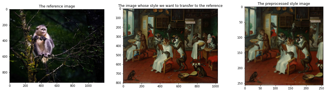
The final_ref_image and the final_style_image (the leftmost and the rightmost images in the canvas below) will be the images we send as the inputs of the model.

1
2
3
4
5
6
7
8
9
10
11
12
13
14
15
16
17
18
19

ref_image_url = "https://upload.wikimedia.org/wikipedia/commons/thumb/0/0d/Black_Snub-nosed_Monkey_(44489823001).jpg/1200px-Black_Snub-nosed_Monkey_(44489823001).jpg"
style_image_url = "https://upload.wikimedia.org/wikipedia/commons/thumb/d/dc/Abraham_Teniers_-_Barbershop_with_monkeys_and_cats.jpg/1024px-Abraham_Teniers_-_Barbershop_with_monkeys_and_cats.jpg"

ref_image = read_image_from_url(ref_image_url)
style_image = read_image_from_url(style_image_url)
final_ref_image = convert_to_float(ref_image)
preprocessed_style_image = preprocess_style_image(style_image)
final_style_image = convert_to_float(preprocess_style_image(preprocessed_style_image))

fig, axs = plt.subplots(1, 3, figsize=(20, 5))
axs[0].imshow(ref_image)
axs[0].set_title("The reference image")

axs[1].imshow(style_image)
axs[1].set_title("The image whose style we want to transfer to the reference")

axs[2].imshow(preprocessed_style_image)
axs[2].set_title("The preprocessed style image")
plt.show()

The API request and response

Here me make a POST request to our model server, sending the “placeholder” and “placeholder_1” inputs we saw earlier.

We use the "instances" and not "inputs" parameter because final_ref_image.tolist() gives a flattened row-wise list.

We send the reference and the style images (a flattened list of them, of course) in the fields "placeholder" and "placeholder_1" of the “instances” list in the json.

We retrieve the "predictions" field from the output, and in its first index we have the output stylized image!

1
2
3
4
5
6
7
8
9
10
11
12
13
14
15

resp = requests.post(
    PREDICTION_ENDPOINT_STYLE,
    json={
        "instances": [
            {
                "placeholder": final_ref_image.tolist(),
                "placeholder_1": final_style_image.tolist(),
            }
        ]
    },
)

# For this particular model, the output image is in the [0] index of the prediction, 
# since we can only render a numpy array as an output image in cv2, we convert it to a numpy array
output_img = np.array(resp.json()["predictions"][0])

The Output!

1
2
3
4
5
6
7
8
9
10
11

fig, axs = plt.subplots(1, 3, figsize=(18, 5))
axs[0].imshow(ref_image)
axs[0].set_title("The reference image")

axs[1].imshow(preprocessed_style_image)
axs[1].set_title("The style image")

axs[2].imshow(output_img)
axs[2].set_title("The stylized image")

plt.show()

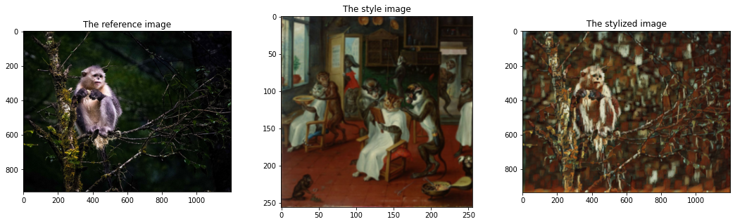
Works pretty swimmingly, as expected!

Serving multiple models

Tensorflow serving also allows us to serve multiple models on the same server.

And doing this is relatively simple! All we have to do is add a config file that defines the models we want to serve.

1
2
3
4
5
6
7
8
9
10
11
12

model_config_list {
    config {
        name: 'super_resolution'
        base_path: '/models/esrgan_super_resolution'
        model_platform: 'tensorflow'
    }
    config {
        name: 'stylization'
        base_path: '/models/magenta_image_stylization'
        model_platform: 'tensorflow'
    }
}

Note that the base_path here is the location of the model inside the docker container, and not on your host system.

Now we can place the config file in the models directory, and simply start the server with the --model_config_file flag, and it will serve the models we defined in the config file.

1
2
3
4

docker run -t -p 8501:8501 \
    -v "$(pwd)/models/:/models/" \
    tensorflow/serving \
    --model_config_file=/models/models.config

Now that we have the super resolution model served up on the same server, let’s see it in action!

Superresolution

Global Variables

1
2
3

PREDICTION_ENDPOINT_SUPER_RESOLUTION = (
    "http://localhost:8501/v1/models/super_resolution:predict"
)

Helper functions

1
2
3
4
5
6
7
8
9
10
11
12

def preprocess_image(image: np.ndarray) -> np.ndarray:
    """
    Resizes the image to the model's input type
    Args:
        image (np.ndarray) : A cv2 COLOR image, BGR

    Returns:
       np.ndarray: a 4D numpy float32 array, compatible with the model's input
    """
    image_float = image.astype(np.float32)
    final_img = np.expand_dims(image_float, axis=0)
    return final_img

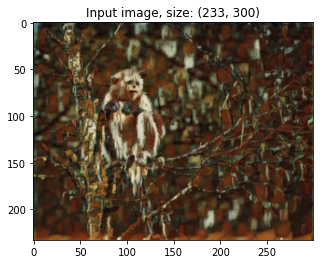
We’ll use a lower quality version of the output of the previous section as the input image

1
2
3
4
5
6
7
8
9
10
11
12
13
14
15
16
17

original_image = output_img.copy()
original_image_shape = original_image.shape[:2]

# purposefully making the image a lower (1/4th) size and changing the type to uint8 so the pixel values fall in the 0-255 range (as accepted by the model)

input_image = (
    cv2.resize(
        original_image,
        (original_image_shape[1] // 4, original_image_shape[0] // 4),
        cv2.INTER_CUBIC,
    )
    * 255
).astype("uint8")

plt.imshow(input_image)
plt.title("Input image, size: {}".format(input_image.shape[:2]))
plt.show()

Preprocessing the image, to make it model-ready, and sending the prediction request to the API

Notice that unlike for the previous model, we are direcly sending the flattened list of the input image in "instances". This is because the model has only one input.

1
2
3
4
5
6
7
8
9

preprocessed_image = preprocess_image(input_image)

resp = requests.post(
    PREDICTION_ENDPOINT_SUPER_RESOLUTION,
    json={
        "instances": preprocessed_image.tolist(),
    },
)
output_image = np.array(resp.json()["predictions"][0]).astype("uint8")

Let’s see the result!

1
2
3
4
5
6
7
8
9
10
11
12
13
14
15
16
17
18
19
20
21
22
23
24
25

output_image = np.clip(
    output_image, 0, 255
)  # a postprocessing step as specified by the superresolution reference paper

fig, axs = plt.subplots(2, 2, figsize=(24, 18))

axs[0][0].imshow(input_image)
axs[0][0].set_title(
    f"The input fed to the superresolution model, size: {input_image.shape[:2]}"
)

axs[0][1].imshow(output_image)
axs[0][1].set_title(
    f"The output of the superresolution model, size: {output_image.shape[:2]}"
)

axs[1][0].imshow(original_image)
axs[1][0].set_title(f"The original image, size:{original_image.shape[:2]}")

axs[1][1].imshow(output_image)
axs[1][1].set_title(
    f"The output of the superresolution model, size: {output_image.shape[:2]}"
)

plt.show()

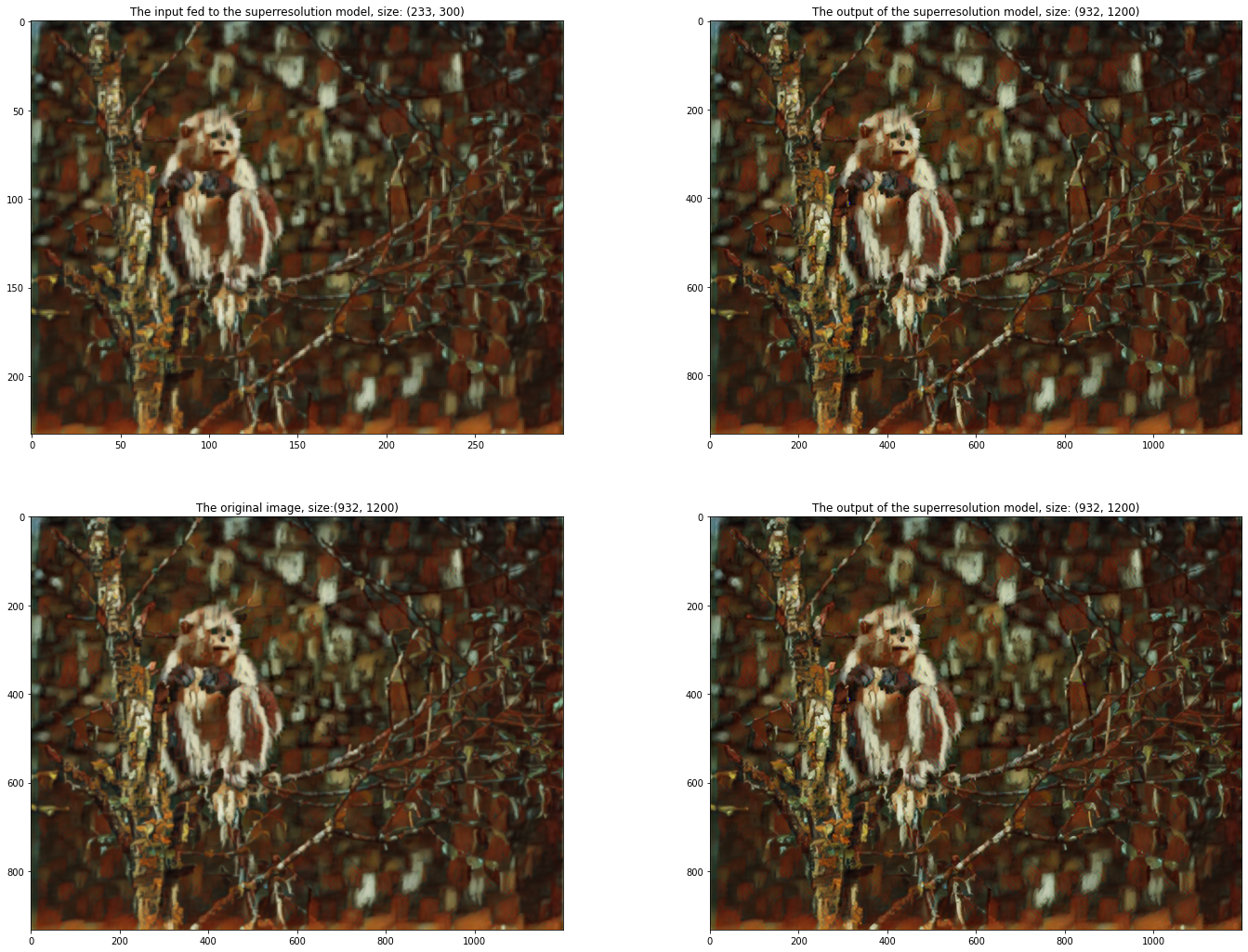
Is it just me, or does the super resolution version look better than the original?

Conclusion

Phew, that was quite the ride wasn’t it?

We have deployed models on the Tensorflow Serving API that we can use to stylize images and enhance an image’s resolution!

We’ve covered the basics of serving models on the Tensorflow Serving API, and this article is just scratching the surface of what tensorflow serving can do. Check out the official guide to check out everything it can do (and it can do a lot)!